Tutorial
This tutorial goes through all the steps required to set up a project, run FishSound Finder and visualize the detections results in Raven.
Setting up the project structure
Create a new folder for your project called Tutorial
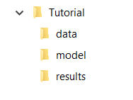
In the Tutorial folder, create with three new subfolders called model, data, and results.
The project folder should look like this:
Downloading the model file
In this example we will run the generic fish sound detector. The classification model is located on FishSound Finder’s GitHub page under the models directory.
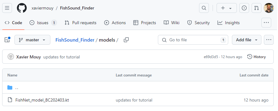
Download the classification model FishNet_model_BC202403.kt from GitHub.
Place the .kt file in your model folder.
Downloading audio data
For this tutorial we will use a single wav file located in the data directory of FishSound Finder’s GitHub page. This audio file was collected off Vancouver Island by an AMAR recorder set with a sampling rate of 32 kHz. The original file was 30-minute long, but was trimmed down for this tutorial. Note that FishSound Finder can interpret timestamp information from the name of the audio files. It currently supports timestamp formats from most popular acoustic recorders including SoundTrap and AMAR.
Download the audio file AMAR173.4.20190920T004248Z.wav from GitHub.
Place it in your data folder.
Creating a deployment file
Creating a deployment file is not necessary but highly recommended. It allows FishSound Finder to embed metadata into the detection results, which makes the post-processing of detection results from multiple recorders much easier. Notice that metadata are included in the NetCDF files generated by FishSound Finder, but not in the Raven files.
Download a deployment file template deployment_info.csv from GitHub.
Place it in your data folder.
Open the deployment_info.csv file with a text editor (e.g. NotePad++) and edit the fields as necessary.
audio_channel_number: [Integer (starting at 1)] Audio channel to being processed.
UTC_offset: [Integer] GMT hour offset of the timestamps in the audio filenames.
sampling_frequency: [Float] Sampling frequency of the audio files in Hz.
bit_depth: [Integer] Bit depth of the audio files.
mooring_platform_name: [String] Short name describing the mooring design (e.g. volumetric array, bottom-mounted).
recorder_type: [String] Name of the acoustic recorder (e.g. SoundTrap 300, AMAR G3).
recorder_SN: [String] Serial number of the acoustic recorder.
hydrophone_model: [String] Model of the hydrophone (e.g. HTI-96).
hydrophone_SN: [String] Serial number of the hydrophone.
hydrophone_depth: [Float > 0] Depth at which the hydrophone was located in meters.
location_name: [string] Name of the deployment locations.
location_lat: [Float] Latitude of the deployment location in decimal degrees.
location_lon: [Float] Longitude of the deployment location in decimal degrees.
location_water_depth: [Float > 0] Water depth at the deployment location in meters.
deployment_ID: [String] Unique name identifying this particular deployment (e.g. SI-RCAIn-20190410).
deployment_date: [String] Date of deployment. Date format: YYYYMMDDTHHMMSS (e.g. 20190410T150155).
recovery_date: [String] Date of recovery. Date format: YYYYMMDDTHHMMSS (e.g. 20190410T150155).
Example of deployment_info file:
deployment_info.csv audio_channel_number
UTC_offset
sampling_frequency
bit_depth
mooring_platform_name
recorder_type
recorder_SN
hydrophone_model
hydrophone_SN
hydrophone_depth
location_name
location_lat
location_lon
location_water_depth
deployment_ID
deployment_date
recovery_date
1
-8
96000
24
bottom weight
SoundTrap 300
1342218252
SoundTrap 300
1342218252
13.4
Snake Island RCA-In
49.21166667
-123.88405
13.4
SI-RCAIn-20190410
20190410T150155
20190625T051114
Running FishSound Finder
Now all the data and configuration files are set up and we can run FishSound Finder. It is here assumed that you are using Anaconda on a Windows machine.
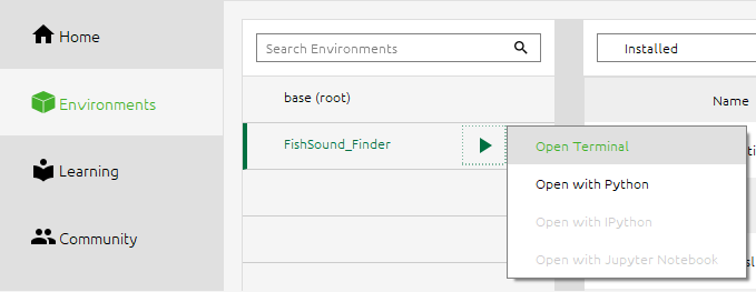
Open Anaconda Navigator
Under the Environments tab on the left, select the python environment in which you installed FishSound Finder (see :ref:’Installation<Installing FishSound Finder>’Installation section), and start a Terminal.
Change the current directory to Tutorial.
$ cd C:\Users\xavier.mouy\Desktop\Tutorial
Start FishSound Finder to process the audio files that are in the data folder.
$ fishsound_finder --audio_folder=".\data" --output_folder=".\results" --model_file=".\models\FishNet_model_BC202403.kt" --threshold=0.995 --deployment_file=".\data\deployment_info.csv"
Alternative: If you don’t want to type the input arguments every time, you can also create a text file with all the input arguments (one per line) and run FishSound Finder using the @ command pointing to that text file.
args_file.txt (saved in the Tutorial folder):
--audio_folder=".\data"
--output_folder=".\results"
--model_file=".\models\FishNet_model_BC202403.kt"
--threshold=0.996
--deployment_file=".\data\deployment_info.csv"
Now running FishSound Finder using args_file.txt.
$ fishsound_finder @.\results\args_file.txt
The console should now display the files being processed and the processing steps in progress.
Namespace(audio_folder='.\data', output_folder='.\results', model='.\model\\FishNet_model_BC202403.kt', threshold=0.996, channel=1, extension='.wav', batch_size=512, step_sec=0.05, smooth_sec=0, min_dur_sec=None, max_dur_sec=None, class_id=1, tmp_dir=None, deployment_file=".\data\deployment_info.csv", deployment_id=None, recursive=False)

1/1: .\data\AMAR173.4.20190920T004248Z.wav
571 detections
Executed in 58.9825 seconds
All files processed in 58.9825 seconds
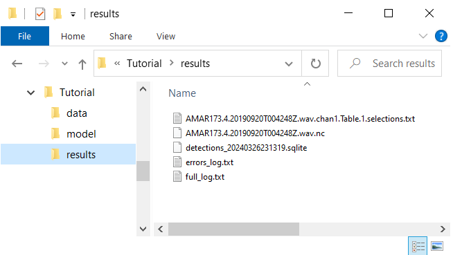
Once FishSound Finder has finished running, all the detection results are written in the results folder. In this case, it created the default netCDF4 file (AMAR173.4.20190920T004248Z.wav.nc) and a Raven file (AMAR173.4.20190920T004248Z.wav.chan1.Table.1.selections.txt), and a SQLite file (detections_20240326231319.sqlite). The SQLite file is a SQL database that regroups the detection results from all files that have been processed. It can be opened using with a software like SQLiteStudio.
Here we only used a single audio file, but note that FishSound Finder will process all audio files located in the data folder. Also note that if the processing is interupted, you can rerun FishSound Finder uisng the same arguments and it will start the processing where it left off (i.e. without reprocessing the files already analized).
Reviewing the processing logs
It is important to review the processing logs once FishSound Finder has finished running to ensure there was no errors. Two log files are automatically created in the results folder:
errors_log.txt: Lists all errors that occurred. An empty file indicates no errors occurred.
full_log.txt: Lists all the information displayed during the processing (including processing times and warning messages).
Analyzing the detection results (documentation in progress)
Detection results from FishSound Finder can be analyzed using the bioacoustics software Raven or libraries such as the ecosound. With the example of the generic fish detector all detections are saved in the output files and are labelled as FS (for a Fish Sound). Each detections has a classification confidence value (comprised between 0 and 1) which can be used to make the detector more or less sensitive depending on the application.
With Raven
To visualize the detection results in Raven:
Open the audio file in Raven
In the File menu, select “Open Sound Selection Table…”, then select the file AMAR173.4.20190920T004248Z.wav.chan1.Table.1.selections.txt from the results folder.
Detection boxes should automatically appear. Notice the confidence value in the selection table.
With ecosound
Here are some code snippets that can be used to analyze the detection results with ecosound. While ecosound can import data from Raven, it is typically better to import the netCDF4 file, as it contains all the metadata for each detections.
Example 1: Display a summary of the detections
from ecosound.core.measurement import Measurement
detection_file = r".\results\AMAR173.4.20190920T004248Z.wav.nc"
detec = Measurement()
detec.from_netcdf(detection_file)
detec.summary()